Transfer Learning

My post introducing convolutional neural networks (CNNs) used a dataset with photos of Arctic foxes, polar bears, and walruses to train a CNN to recognize Artic wildlife. Trained with 300 images – 100 for each of the three classes – the CNN achieved an accuracy around 60%. That’s not sufficient for most purposes. Imagine you’re a climate scientist tracking polar bears in the wild, and you’re using AI to analyze photos snapped by motion-activated cameras to determine which ones contain polar bears. 60% accuracy won’t get you very far.

One solution is to train the CNN with tens of thousands of photos. A better solution – one that can deliver world-class accuracy with the 300 photos you have and doesn’t require expensive GPUs – is transfer learning. In the hands of software developers and engineers, transfer learning makes CNNs a practical solution for a variety of computer-vision problems. And it requires orders of magnitude less time and compute power than CNNs built from scratch. Let’s take a moment to understand what transfer learning is and how it works – and then put it to work finding polar bears.

Understanding Transfer Learning

Pretrained CNNs trained on the ImageNet dataset can identify Arctic foxes and polar bears, but as demonstrated in my previous post, they can’t detect walruses because they weren’t trained with walrus photos. Transfer learning lets you repurpose pretrained CNNs to identify objects they weren’t originally trained to identify. It leverages the intelligence baked into pretrained CNNs, but it redirects that intelligence to solve domain-specific problems.

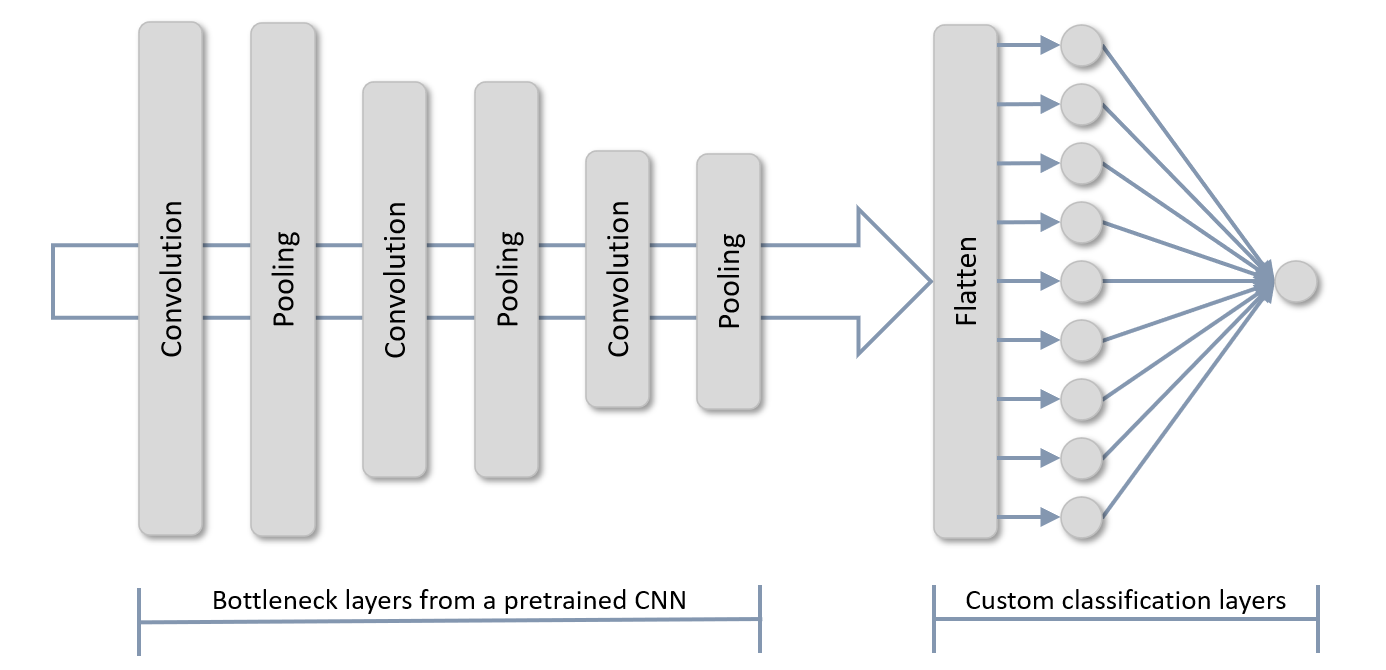
Recall that a CNN contains two groups of layers: bottleneck layers (also known as feature-extraction layers) containing the convolution and pooling layers that extract features from images at various resolutions, and classification layers, which classify features output from the bottleneck layers as belonging to an Arctic fox, a polar bear, or something else. The convolution layers use matrices called convolution kernels to extract features, and the values in the convolutional kernels are learned during training. This learning accounts for the bulk of the training time. When sophisticated CNNs are trained with millions of images, the convolution kernels become very efficient at extracting features.

The premise behind transfer learning is shown below. You load the bottleneck layers of a pretrained CNN, but you don’t load the classification layers. Instead, you provide your own, which train orders of magnitude more quickly than an entire CNN. Then you pass the training images through the bottleneck layers for feature extraction, and train the classification layers on those features. The pretrained CNN might have been trained to extract features from pictures of apples and oranges, but those same layers are probably pretty good at extracting features from photos of dogs and cats, too. By using the pretrained bottleneck layers to do feature extraction and then using those features to train your own classification layers, you can teach the model that a certain feature extracted from an image might be indicative of a dog rather than an apple.

---

---

Transfer learning is relatively simple to implement with Keras and TensorFlow. Recall that the following statement loads Microsoft’s ResNet50V2 CNN and initializes it with the weights (including kernel values) that were arrived at when the network was trained on a subset of the ImageNet dataset:

To load ResNet50V2 (or any other pretrained CNN that Keras supports) without the classification layers, you simply add an include_top=False attribute:

From that point, there are two different ways to implement transfer learning. The first involves appending classification layers to the base model’s bottleneck layers, and setting each base layer’s trainable attribute to False so the convolution kernels won’t be updated when the network is trained:

The second technique is to run all the training images through the base model for feature extraction, and then run the features through a separate network containing your classification layers:

Which technique is better? The second is faster because the training images go through the bottleneck layers for feature extraction just one time rather than once per epoch. It’s the technique you should use in the absence of a compelling reason to do otherwise. The first technique is slightly slower, but it lends itself to fine tuning, in which you unfreeze one or more of the bottleneck layers after training is complete and train for a few more epochs with a very low learning rate. It also makes it easy to perform data augmentation, which I’ll introduce in my next post.

Because no training is done in the bottleneck layers when the network is trained, transfer learning is much faster than training a sophisticated CNN. And because the bottleneck layers were trained when the pretrained CNN was trained, they’re already adept at extracting features from images.

If you use the first technique above to implement transfer learning, you make predictions by preprocessing the images and passing them to the model’s predict method. If you use the second (faster) technique, making predictions is a 2-step process. After preprocessing the images, you pass them to the base model’s predict method, and then you pass the output from that method to your model’s predict method:

And with that, transfer learning is complete. All that remains is to put it in practice.

Use Transfer Learning to Identify Arctic Wildlife

Let’s use transfer learning to solve the same problem that we attempted to solve with a scratch-built CNN in my post introducing CNNs: building a model that determines whether a photo contains an Arctic fox, a polar bear, or a walrus.

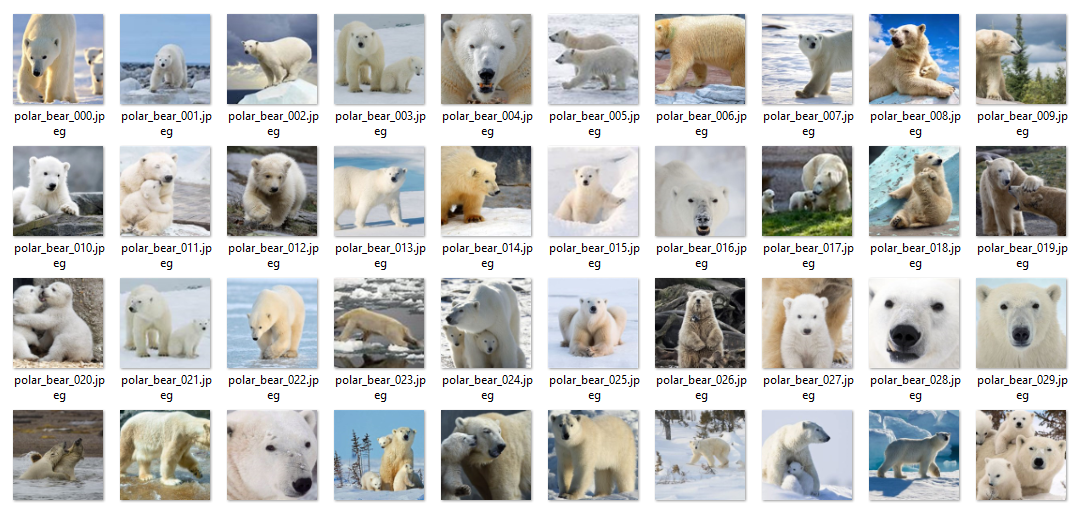
Start by downloading the zip file containing Arctic wildlife images if you haven’t downloaded it already. Unpack the zip file and place its contents in the directory where your Jupyter notebooks are hosted. The zip file contains folders named “train,” “test,” and “samples.” Each folder contains subfolders named “arctic_fox,” “polar_bear,” and “walrus.” The training folders contain 100 images each, while the test folders contain 40 images each. Here again are some of the polar-bear training images.

---

---

As you did in the earlier tutorial, create a Jupyter notebook and paste the following code into the first cell to define helper functions for loading and labeling images and declare Python lists for accumulating images and labels:

Use the following statements to load 100 Arctic-fox training images and plot a subset of them:

Load and label the polar-bear training images:

And then the walrus training images:

We also need to load the images used to validate the CNN. Start with 40 Arctic-fox test images:

Then the polar-bear test images:

And finally, the walrus test images:

Now that the training and test images are loaded and labeled, the next step is to one-hot-encode the labels and preprocess the images. We’ll be using ResNet50V2 as our pretrained CNN, so we’ll use the ResNet version of preprocess_input to preprocess the pixels, and then divide each pixel value by 255:

The next step is to load a pretrained CNN, being careful to load the bottleneck layers but not the classification layers, and use it to extract features from the training and test images:

Now we’ll train our own neural network to classify features extracted from the training images:

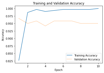
How well did the network train? Plot the training accuracy and validation accuracy for each epoch:

Your results will differ from mine, but I got about 95% accuracy. If you didn’t quite get there, try training the network again:

Finally, use a confusion matrix to visualize just how well the network is able to distinguish the various classes:

To see transfer learning at work, load one of the Arctic-fox images from the “samples” folder. That folder contains wildlife images that the model was neither trained nor tested with:

Now preprocess the image, run it through ResNet50V2‘s feature-extraction layers, and run the output through the newly trained classification layers:

With a little luck, the network predicted with almost 100% confidence that the image contains an Arctic fox. Perhaps that’s not surprising since ResNetV2 was trained with Arctic-fox images as well as polar-bear images. But now let’s load a walrus image, which, you’ll recall, ResNet50V2 was unable to classify:

Preprocess the image and make a prediction:

ResNet50V2 wasn’t trained to recognize walruses, but our network was. That’s transfer learning in a nutshell. It’s the deep-learning equivalent of having your cake and eating it, too. And it’s the secret sauce that makes CNNs a viable tool for anyone with a laptop and a few hundred training images.

That’s not to say that transfer learning will always get you 95% accuracy with 100 images per class. It won’t. If a dataset lacks the information to achieve that level of separation, neither scratch-built CNNs nor transfer learning will magically make it happen. That’s always true in machine learning and AI. You can’t get water from a rock. And you can’t build an accurate model from data that doesn’t support it.

Get the Code

You can download a Jupyter notebook demonstrating transfer learning from the deep-learning repo that I maintain on GitHub. Feel free to check out the other notebooks in the repo while you’re at it. Also be sure to check back from time to time because I am constantly uploading new samples and updating existing ones.